Who is that Neural Network?

Henrique M. Soares

Independent researcher. São Paulo, SP, Brazil.

Email: hemagso (at) gmail (dot) com

Pokémon has been an enormous success around the globe for more than 20 years. In this paper, I tackle the “Who’s that Pokémon?” challenge from a machine learning perspective. I propose a machine learning pre-processing and classification pipeline, using convolutional neural networks for classification of Pokémon sprites.

COMPUTING AND IMAGE RECOGNITION

Since they were invented^[1], computers became increasingly present in our everyday life. Initially restricted to mathematical problem-solving and military applications in ballistics and cryptography, their applications become more diverse by the minute. As of today, machines beat humans in lots of tasks, one of the most recent being AlphaGo’s victory over the Go world champion (Go Game Guru, 2017).

This achievement is a testament to the remarkable advances sustained by machines towards intelligent applications. Go, with its almost infinite combinations^[2], is not an easy problem to solve by “brute force”^[3], the strategy usually employed by computers against humans in other perfect information games.

But do not despair, for not all is lost in our fight against our future robot overlords, as computers still struggle with a task that humans were quite literally born to do: image and pattern recognition. However good a computer may be today, humans are still way better at noticing that, even though Figure 1 shows a car, something quite unusual happened to it.

Figure 1. Crashed car against a tree. This text was definitely not written by a robot overlord (yet). (Image extracted from Wikimedia Commons; Thue, 2005).

But computers are catching on! Advances in machine learning techniques, especially in supervised learning methods, and the ever-growing data available for feeding these algorithms have been enabling giant leaps in this field. In 2015, a 150 layers’ residual neural network ensemble, trained by the MSRA team, achieved a 62% average precision in the 2015 image classification challenge with a data set with more than 1,000 different objects (Large Scale Visual Recognition Challenge, 2015).

Figure 2. Some simple things may be hard to a computer. (“Tasks”; XKCD, available from https://xkcd.com/1425).

So, we wonder… How would our machines fare against a challenge tackled by children around the world for the last 22 years?

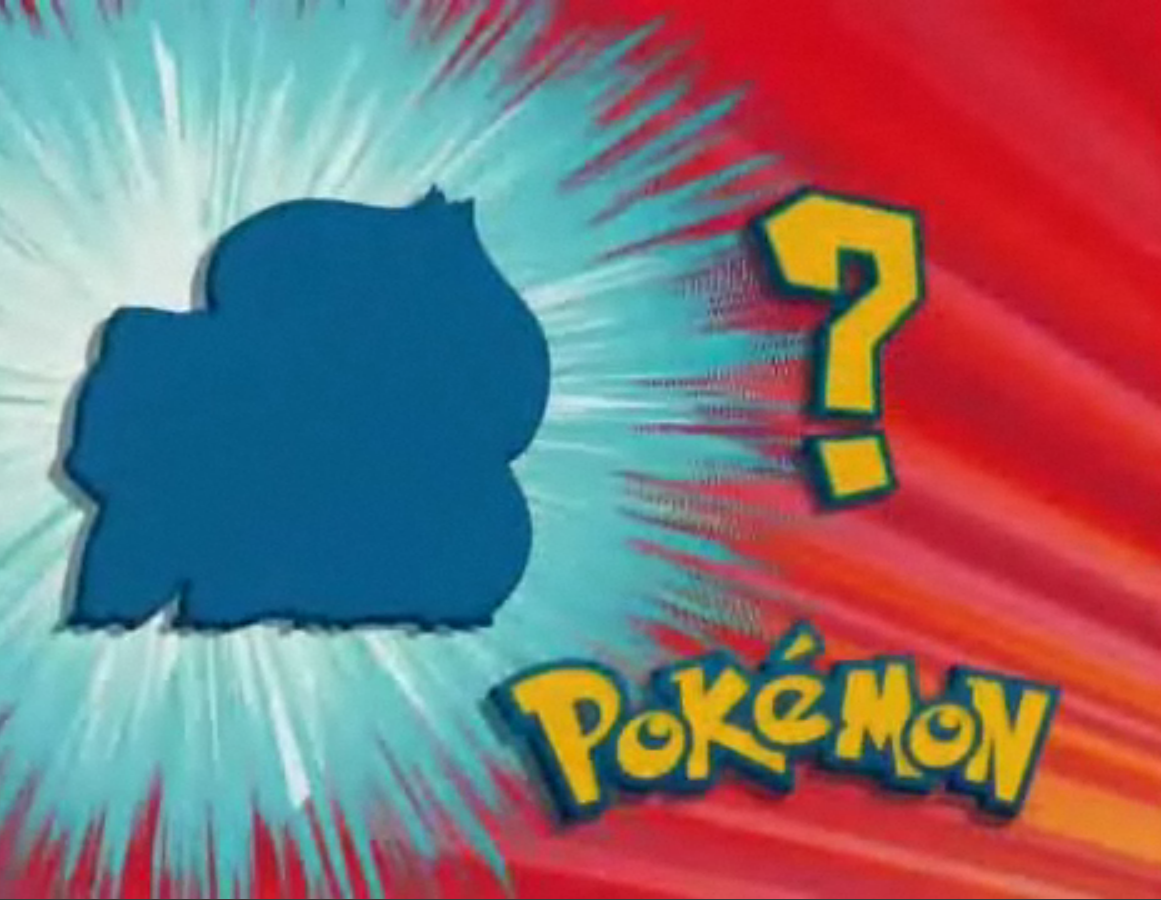
Figure 3. Who’s that Pokémon? (Screenshot from the Pokémon animated series.)

POKÉMON

Pokémon is an extremely successful franchise of games and animated series targeted at young audiences (although some people, as the author, disagree with this classification). The franchise was created by Satoshi Tajiri in 1995, with the publishing of two games for Nintendo’s handheld console Game Boy. In the game, the player assumes the role of a Pokémon trainer, capturing and battling the titular creatures. It was an enormous success, quickly becoming a worldwide phenomenon (Wikipedia, 2017b).

The franchise started with a total of 151 monsters (Fig. 4), but today the games have reached their seventh iteration, counting with a total of 802 monsters.

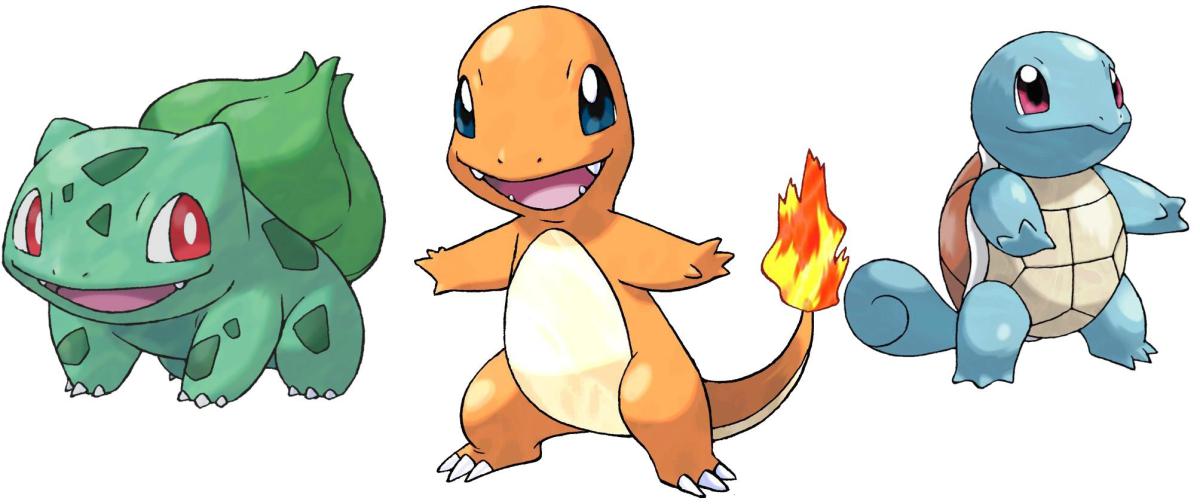
Figure 4. Left to right: Bulbasaur, Charmander and Squirtle. (Official art by Ken Sugimori; image taken from Bulbapedia, 2017).

Each Pokémon belongs to one or two types indicating its “elemental affinity”, as well as its strengths and weakness against other types. This feature is essential to the gameplay, establishing a deep and complex rock-paper-scissor mechanic that lays at the foundation of the combat system. There are 18 types (they were only 15 in the first game), as seen in Figure 5 (Bulbapedia, 2017).

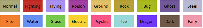
Figure 5. The 18 Pokémon types, depicted with their usual background colors.

In this paper, I examine the performance of convolutional neural networks (also known as ConvNets) in a Pokémon Type classification task given a Pokémon game sprite. I will present the data collected, the pre-processing and training pipelines, ending with the performance metrics of the selected model. All the data, implementation code and results, as well as a Jupyter Notebook with the explanation of all the steps, are available in a GitHub repository (https://github.com/hemagso/Neuralmon).

DATA PREPARATION

Dataset Features

To train the models, I am going to use game sprites. The dataset (the sprite packs) was obtained at Veekun (2017). These packs contain sprites ripped from the games’ so-called generations 1 to 5. Although there have been new games (and new monsters) released since then, they use tridimensional animated models; making it harder to extract the resources from the games, as well as making it available in a format that can be fed to a machine learning method. As such, in this paper we will only use Pokémon up until the fifth generation of the games (649 in total).

Figure 6 depicts the sprites of the three first-generation starters throughout all the games considered in this study.

We can immediately see that detail level varies between games, due to the different hardware and capabilities of the gaming consoles. The first generation, released for Nintendo’s Game Boy, has almost no hue variation in a single sprite, although there is some hue information in the dataset (for instance, Bulbasaur is green, Charmander is red and Squirtle is blue; Fig. 6). As we go on, through Game Boy Advance to Nintendo DS, we see that the level of detail skyrockets, not only in terms of hue, but also in shapes.

At a first glance, we can also identify some typical problems encountered in image classification tasks. The images have different sizes. Even though the Aspect Ratio in all images stays at a one-to-one ratio, we have images ranging from 40-pixel width in the first generation to 96-pixel width in the fifth one (pay attention to the scales on the border on each sprite in Figure 6).

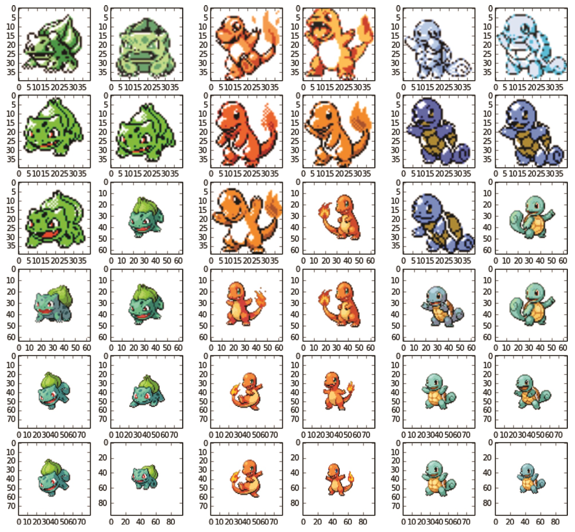
Figure 6. Example of the variation of the sprites for three Pokémon, as seen throughout games and generations.

Also, not all sprites fill the same space in each image. Sprites from the oldest generations seem to fill, in relative terms, a bigger portion of their images. This also happens within the same generation, especially in newer games, relating, in general, to the differences in size of each Pokémon and its evolutions (Fig. 7).

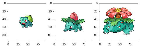
Figure 7. Bulbasaur’s evolutionary line, as seen in the game’s 5^th generation. As the Pokémon evolves and gets larger, its sprite fills up a larger portion of the image.

Image Centering

To solve this problem, let’s apply some computer vision techniques to identify the main object in the image, delimitate its bounding box and center our image on that box. The pipeline for that is:

Convert the image to grayscale.
Apply a Sobel Filter on the image, highlighting the edges of the sprite. The Sobel filter is a 3×3 convolutional kernel (more about these handy little fellows later, but see also Sckikit-Image, 2017) that seeks to approximate the gradient of an image. For a given image ‘A’, the Sobel operator is defined as:

Fill the holes in the image, obtaining the Pokémon’s silhouette.
Calculate the Convex Hull of the silhouette, that is, the smallest convex polygon that includes all pixels from the silhouette.
Define the square bounding box from the convex hull calculated before.
Select the content inside the bounding box, and resize it to 64 x 64 pixels.

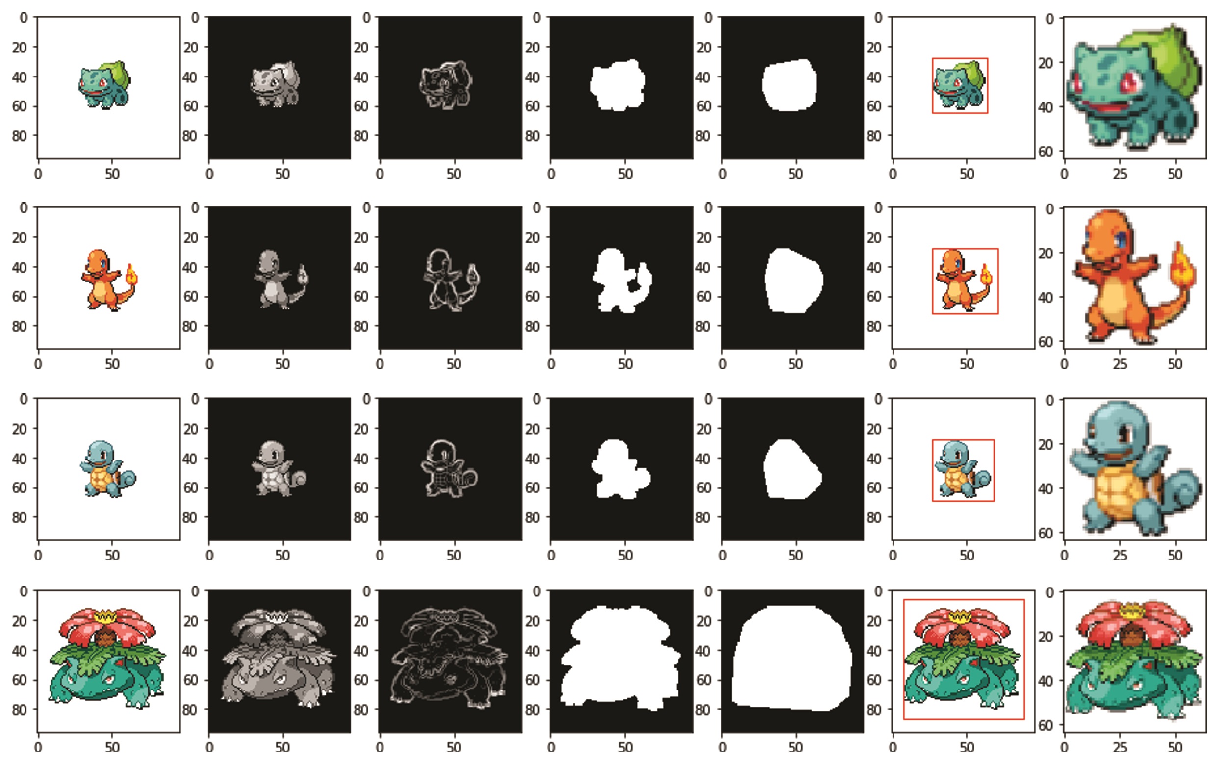
Figure 8. Examples of all steps of the sprite centering pipeline.

After following the pipeline outlined above, we obtain new sprites that maximize the filling ratio of the sprite on the image. Those steps were taken using skimage, an image processing library for the Python programming language. Figure 8 shows the results of our pipeline for the sprites of the three 1^st generation starters and Venusaur.

Our proposed pipeline is extremely effective at the task at hand. That is to be expected, as our images are very simple sprites, with a very clear white background.

Finally, let’s apply our method on all our monsters and images. Figure 9 shows the results for a bunch of Pokémon.

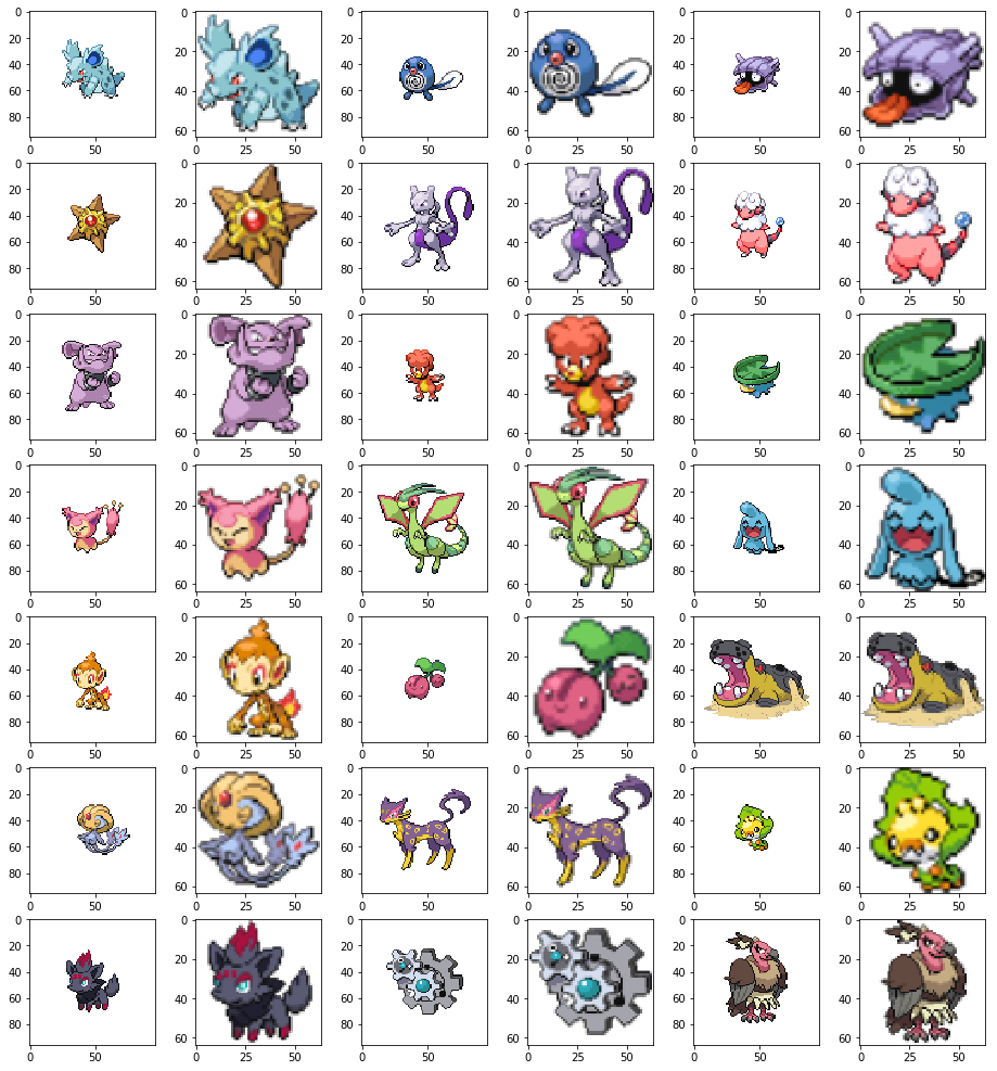
Figure 9. Centering results over various 5^th gen Pokémon.

Target Variable

Now that we have all our Pokémon images to build our image dataset, we have to classify them in accordance with the variable that we want to predict. In this paper, we will try to classify each Pokémon according to its correct type using only its image. For example, in Figure 10 we try to use the image inside the bounding box to classify the Pokémon in one of the 18 types, trying to match its true type (shown below each Pokémon).

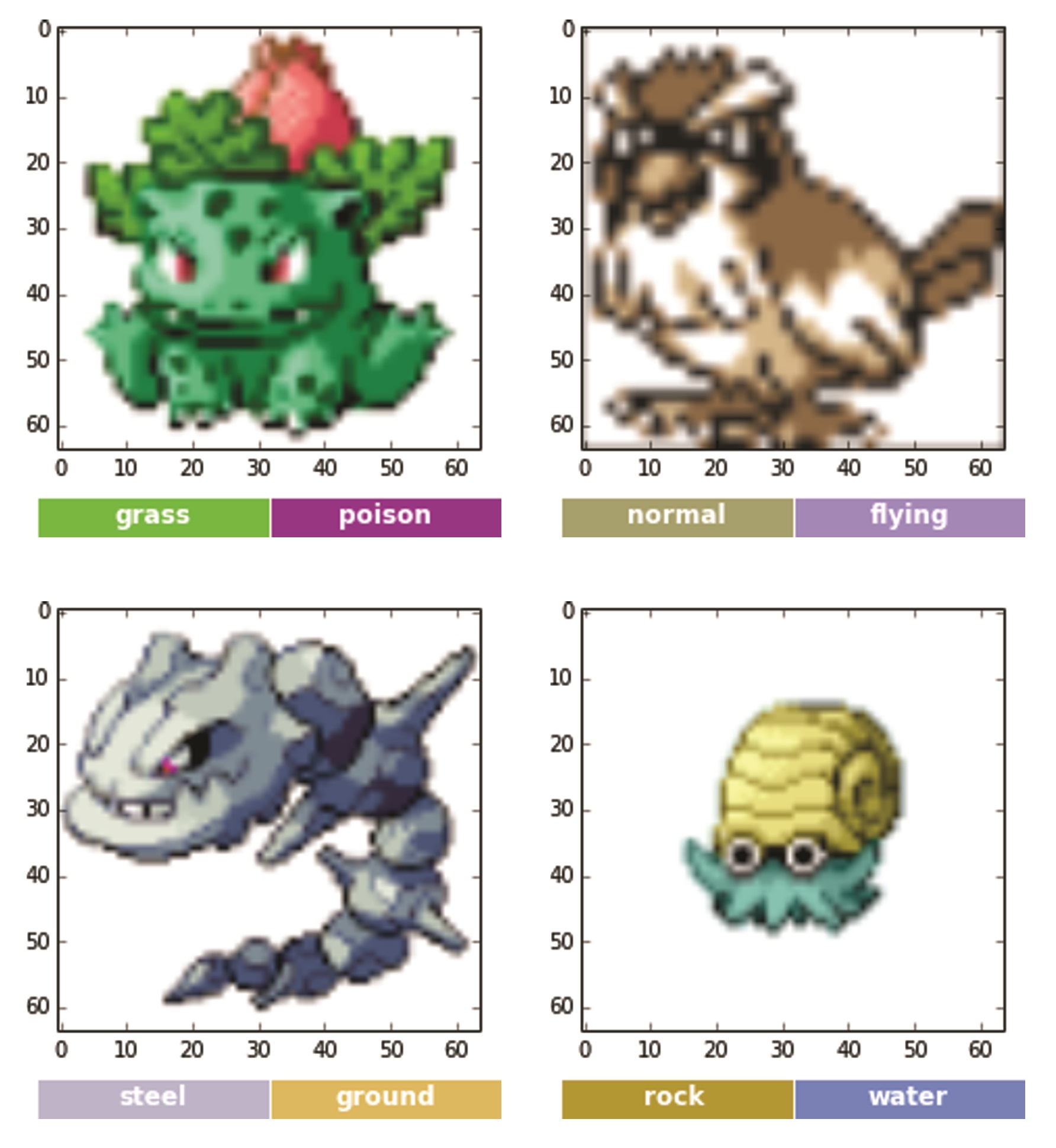
Figure 10. Example Pokémon and their respective types. Top row: Ivysaur (left) and Pidgey (right). Bottom row: Steelix (left) and Lord Helix (right), praise be unto him.

But there is a catch. A significant portion of the Pokémon, like all those from Figures 9 and 10, have a dual type. That is, its true type will be a combination of two different types from that list of 18 types. In Figure 10, for instance, Ivysaur is both a Grass type and Poison type, and has the strengths and weakness of both types.

To take this into account, we would have to make our target classifications over the combination of types. Even if we disregard type order (that is, consider that a [Fire Rock] type is the same class as a [Rock Fire] one), we would end up with 171 possible classes. (Actually, this number is a little bit smaller, 154, as not all combinations exist in the games.)

To make things worse, some combinations are rare (Fig. 11), with only one or two Pokémon, thus limiting the available samples to learn from.

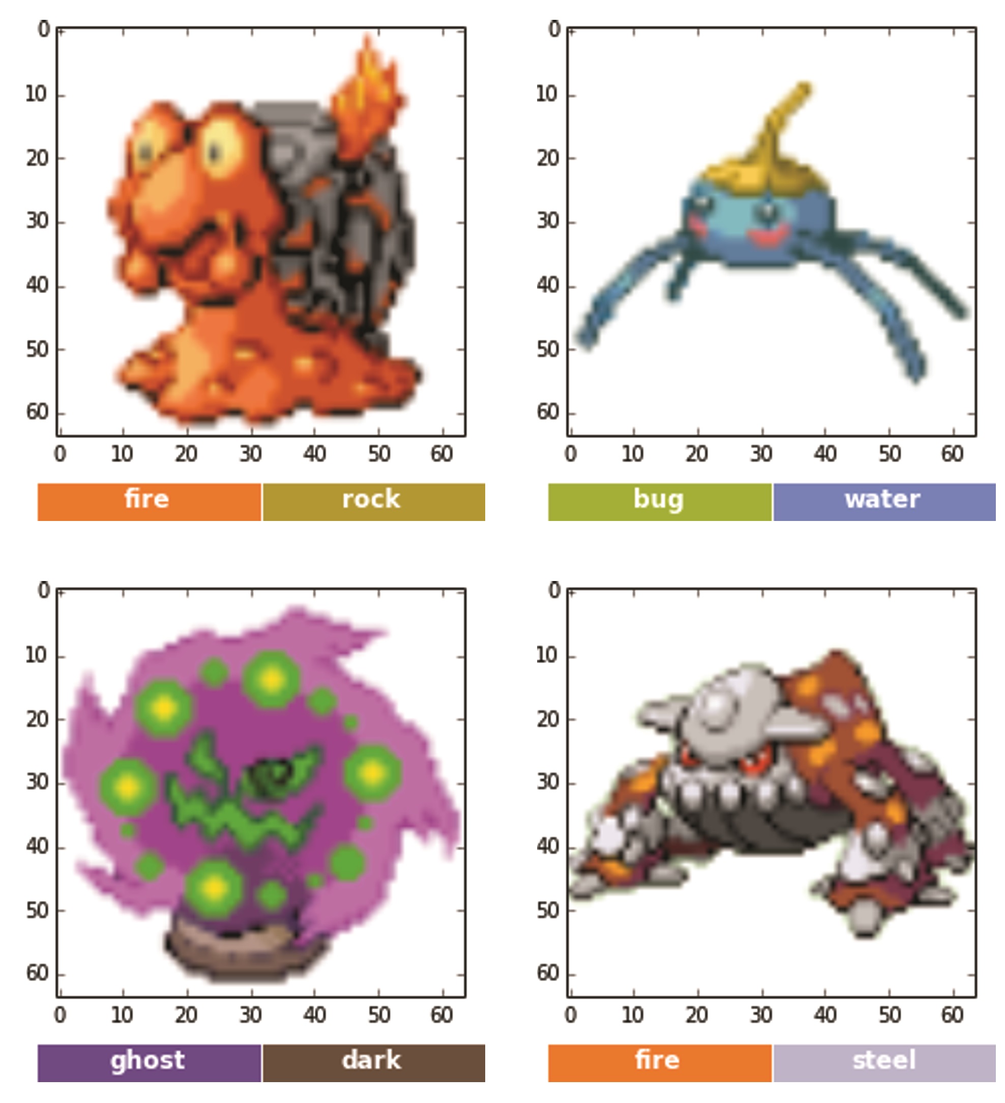
Figure 11. Some unique type combinations. Top row: Magcargo (left) and Surskit (right). Bottom row: Spiritomb (left) and Heatran (right).

Due to the reasons outlined above, I opted to disregard type combinations in this paper. As such, we are only taking into account the primary type of a Pokémon. For instance, in Figure 10 we would have: Ivyssaur: Grass; Pidgey: Normal; Steelix: Steel; Lord Helix: Rock.

MODEL TRAINING

Chosen Model

I used a convolutional Neural Network as a predictor on our dataset. Neural networks are one among many kinds of predictive models usually used in machine learning, consisting of an interconnected network of simple units, known as Neurons. Based on a loose analogy with the inner workings of biological systems, Neural Networks are capable of learning complex functions and patterns through the combination of those simple units (Wikipedia, 2017a).

In its simplest form, a Neuron is nothing more than a linear function of its inputs, followed by a non-linear activation function (Fig. 12). However, through the combination of several layers, neural networks are capable of modelling increasingly complex relationships between the independent and dependent variables at hand (Fig. 13).

Figure 12. The basic unit of a Neural Network.

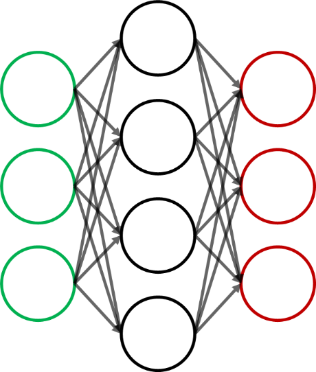
Figure 13. A slightly more complex architecture for a neural network, with one hidden layer.

Neural networks are not exactly new, as research exists since 1940 (Wikipedia, 2017a). However, only with recent computational advances, as well as the development of the backpropagation algorithm for its training, that its use became more widespread.

OK, this is enough to get us through the Neural Network bit. But what the hell “convolutional” means? Let’s first talk a little about Kernels.

In image processing, a Kernel (also known as Convolution Matrix or Mask) is a small matrix used in tasks as blurring, sharpening, edge detection, among others. The effect is obtained through the calculation of the matrix convolution against the appropriate Kernel, producing a new image. We have already seen a Kernel used in this paper, in our pre-processing pipeline, where we applied a Sobel Kernel to detect the edges of a sprite.

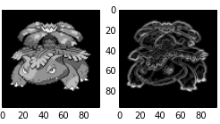
Figure 14. Sobel Kernel effect on Venusaur’s sprite.

The convolution operation may be thought of as a sliding of the Kernel over our image. The values in the Kernel multiply the values below them in the image, element-wise, and the results are summed to produce a single value of the convolution over that window. (A much better explanation about the convolution operation can be found at http://setosa.io/ev/ image-kernels/.) In Figure 15, we apply a vertical Sobel filter to detect sharp variations in color intensity (ranging in our grayscale images from 120 to 255).

Figure 15. Convolution example. The red area highlighted in the image is being convoluted with a Vertical Edge detector, resulting in the red outlined value on the resulting matrix.

But what the heck! What do those Kernels have to do with neural networks? More than we imagine! A convolutional layer of a neural network is nothing more than a clever way to arrange the Neurons and its interconnections to achieve an architecture capable of identifying these filters through supervised learning. (Again, a way better explanation about the whole convolutional network-stuff may be found in http://cs231n.github.io/convolutional-network s/.) In our pre-processing pipeline, we used a specific Kernel because we already knew the one that would excel at the task at hand, but in a convolutional network, we let the training algorithm find those filters and combine them in subsequent layers to achieve increasingly complex features.

Our Neural Network’s Architecture

I used a small-depth convolutional network for our Pokémon classification task (Fig. 16).

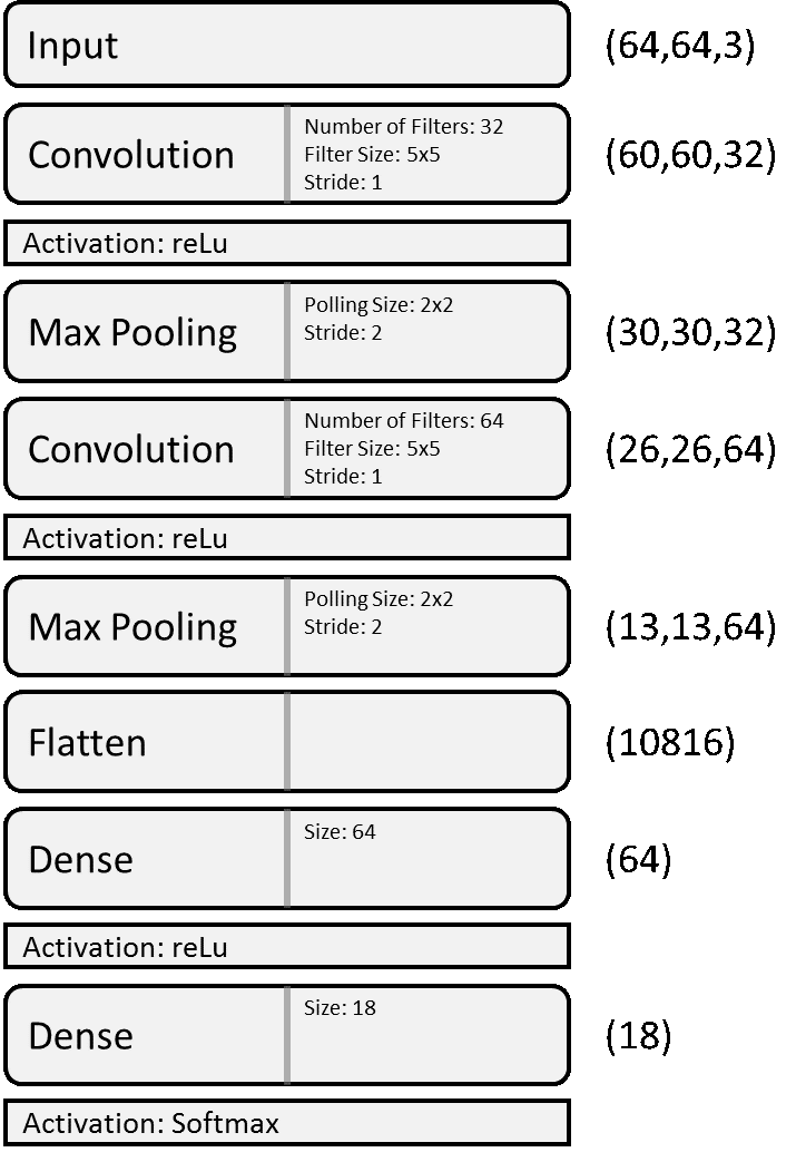
Figure 16. Architecture of the Neural Network used here.

Each layer of the image represents a layer in our convolutional network. After each layer, we obtain a state tensor that represents the output of that layer (the dimension of the tensor is listed on the right side of each layer).

A convolution layer then applies the convolution operation. In the first layer, we apply 32 kernels of size 5 to the input image, producing 32 outputs of size 60 x 60 (with each convolution the image size diminishes due to border effects).

We also use max polling layers that simply reduce a tensor region to a single one by getting its maximum value (Fig. 17). As such, after the application of a 2 x 2 max polling layer, we get a tensor that is a quarter of the size of the original.

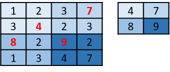
Figure 17. Example of the max pooling operation.

At the end, we flatten our tensor to one dimension, and connect it to densely connected layers for prediction. Our final layer has size 18, the same size as the output domain.

Train and Validation

To achieve our model training we are going to split our dataset in two parts: (1) the ‘training dataset’ will be used by our training algorithm to learn the model parameters from the data; (2) the ‘validation dataset’ will be used to evaluate the model performance on unseen data. In this way, we will be able to identify overfitting issues (trust me, we are about to see a lot of overfitting^[4]).

But we can’t simply select a random sample of our sprites. Sprites from the same Pokémon in different games are very similar to each other, especially between games of the same generation (Fig. 18).

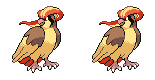
Figure 18. Sprites of Bird Jesus from Pokémon Platinum (left) and Diamond (right). Wait… was it the other way around?

Box 1. Performance Metrics

In this article, we used three performance metrics to assess our model performance:

(1) Accuracy: the percentage of predictions that got the right type classification of the Pokémon;

(2) Precision: the percentage of images classified as a class (type) that truly belonged to that class;

(3) Recall: the percentage of images of a class (type) that were classified as that class.

While accuracy enable us to get an overall quality of our model, precision and recall are used to gauge our model’s prediction of each class.

If we randomly select sprites, we incur on the risk of tainting our validation set with sprites identical to the ones on the training set, which would lead to a great overestimation of model performance on unknown data. As such, I opted for Pokémon-wise sample. That is, I assigned the whole Pokémon to a set, instead of assigning individual sprites. That way, if Charizard is assigned to the validation set, all its sprites would follow, eliminating the risk of taint.

I used 20% of the Pokémon for the test sample, and 80% for the training set, which leaves us with 2,727 sprites for training.

First Model: Bare Bones Training

For the first try, I fed the training algorithm the original sprites, while keeping the training/ validation split. The algorithm trained over 20 epochs^[5], which took about a minute in total^[6]. The results obtained in this first training session are presented in Figure 19 (see also Box 1 for an explanation of the performance metrics).

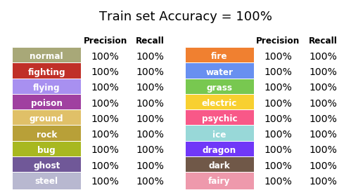
Figure 19. Performance of the training set in the first try.

Impressive! We got all the classifications right! But are those metrics a good estimation of the model performance over unseen data? Or are those metrics showing us that our models learned the training sample by heart, and will perform poorly on new data? Spoiler alert: it will. Let’s get a good look at it: Figure 20 exhibits those same metrics for our validation set.

It seems that our model is indeed overfitting the training set, even if it’s performing better than a random guess.

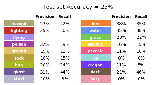
Figure 20. Performance of the validation set in the first try.

But wait a minute… why haven’t we got any Flying type Pokémon? It turns out that there is only one monster with Flying as its primary type (Tornadus; Fig. 21), and he is included in the training set.

Figure 21. Tornadus is forever alone in the Flying type.

Second Model: Image Augmentation

The poor performance our first model obtained for the validation set is not a surprise. Image classification, as said in the introduction, is a hard problem for computers to tackle. Our dataset is too small and does not have enough variation to enable our algorithm to learn features capable of generalization over a wider application.

To solve at least part of the problem, let’s apply some image augmentation techniques. This involves applying random transformations over the training images, thus enhancing their variation. A human being would be able to identify a Pikachu, no matter its orientation (upside down, tilted to the side etc.) and we would like our model to achieve the same. As such, I applied the following range of transformations over our training dataset (Fig. 22): (1) random rotation up to 40 degrees; (2) random horizontal shifts up to 20% image width; (3) random vertical shifts up to 20% image height; (3) random zooming up to 20%; (4) reflection over the vertical axis; and (5) shear transformation over a 0.2 radians range.

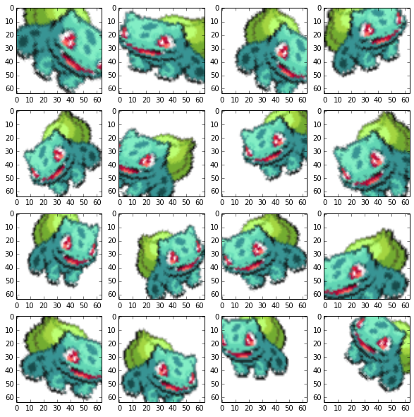
Figure 22. Images obtained through the image augmentation pipeline for one of Bulbasaur’s sprites.

I applied this pipeline to all sprites in our training set, generating 10 new images for each sprite. This way, our training set was expanded to 27,270 images. But will it be enough? After training over 30 epochs (this time it took slightly longer, a little over 10 minutes in total), I obtained the following results (Fig. 23).

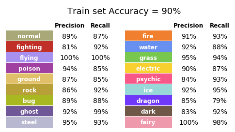
Figure 23. Performance of the training set for the second model.

Wait a minute, has our model’s performance decreased? Shouldn’t this image augmentation thing make my model better? Probably, but let’s not start making assumptions based on our training set performance. The drop in overall performance is due to the increase in variation in our training set and this could be good news if it translates into a better performance for the validation set (Fig. 24).

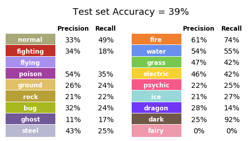
Figure 24. Performance of the validation set for the second model.

And here we have it! Image augmentation actually helped in the model’s performance. The accuracy was raised by 14 percentage points, to a total of 39%. We could keep trying to get a better model, fiddling with model hyper-parameters or trying net architectures, but we are going to stop here.

Taking a Closer Look on the Classifications

There are some things that I would like to draw your attention to. The types with greater prediction Accuracy are: Fire (61%), Water and Poison (54% each), Grass (47%), Electric (46%). The types with greater Recall (see Box 1) are: Dark (92%), Fire (74%), Water (55%), Normal (49%), Grass (42%).

It’s no surprise that the three main types (Fire, Water and Grass) are among the top five in both metrics. These types have very strong affinities with colors, an information easily obtained from the images. They also are abundant types, having lots of training examples for the model to learn from.

Now let’s look at some correctly and incorrectly classified Pokémon (Figs. 25 and 26, respectively).

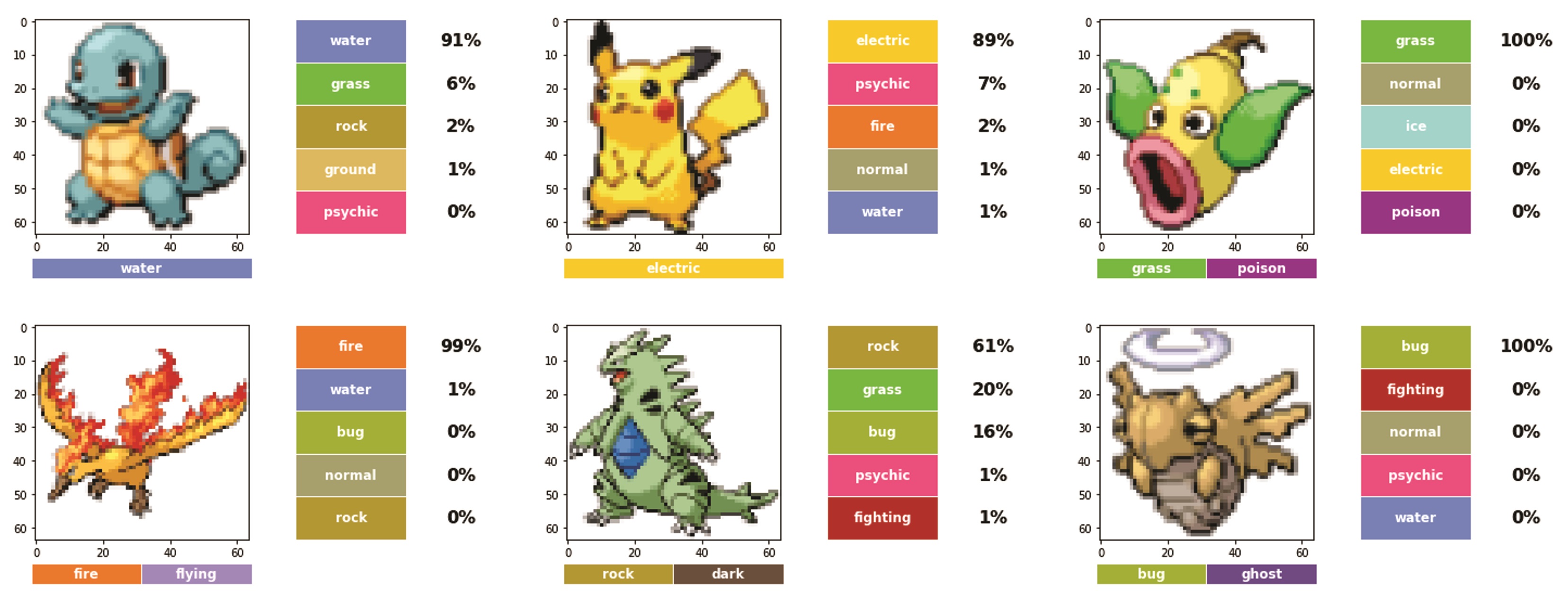
Figure 25. Some correctly classified Pokémon. Top row: Squirtle (left), Pikachu (center), Weepingbell (right). Bottom row: Moltres (left), Tyranitar (center), Shedinja (right).

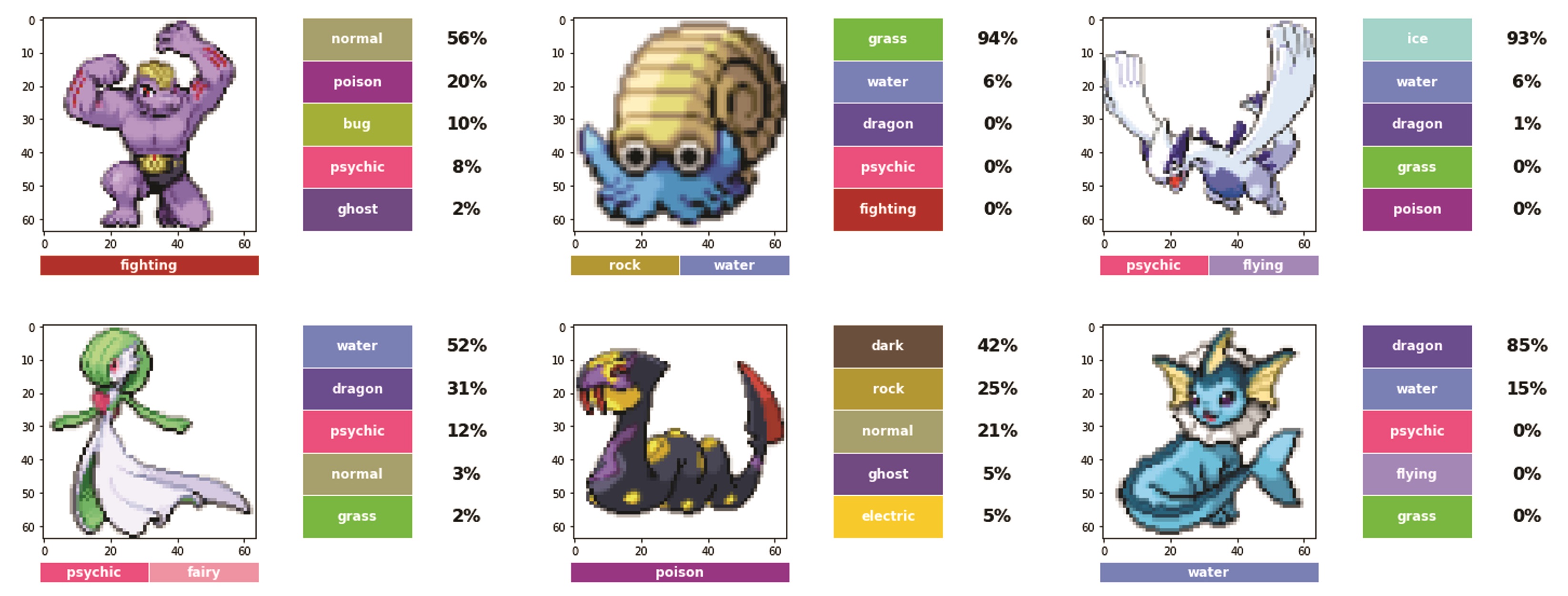
Figure 26. Some incorrectly classified Pokémon. Top row: Mochoke (left), Our Good Lord Helix (center), Lugia (right). Bottom row: Gardevoir (left), Seviper (center), Vaporeon (right).

Even in this small sample, we can see that color plays an important part in the overall classification. For example, in the incorrectly-classified Pokémon, Machoke had good chances of being a Poison type, possibly due to its purple color. Likewise, Seviper was classified as a Dark type probably due to its dark coloration.

And why is that? Well, we may never know! One of the downsides of using deep neural networks for classification is that the model is kind of a “black box”. There is a lot of research going on trying to make sense of what exactly is the network searching for in the image. (I recommend that you search the Internet for “Deep Dream” for some very trippy images.)

For now, we can look at the first layer activations for some of the Pokémon and try to figure out what is it that each kernel is looking for. But as we go deeper into the network, this challenge gets harder and harder (Fig. 27).

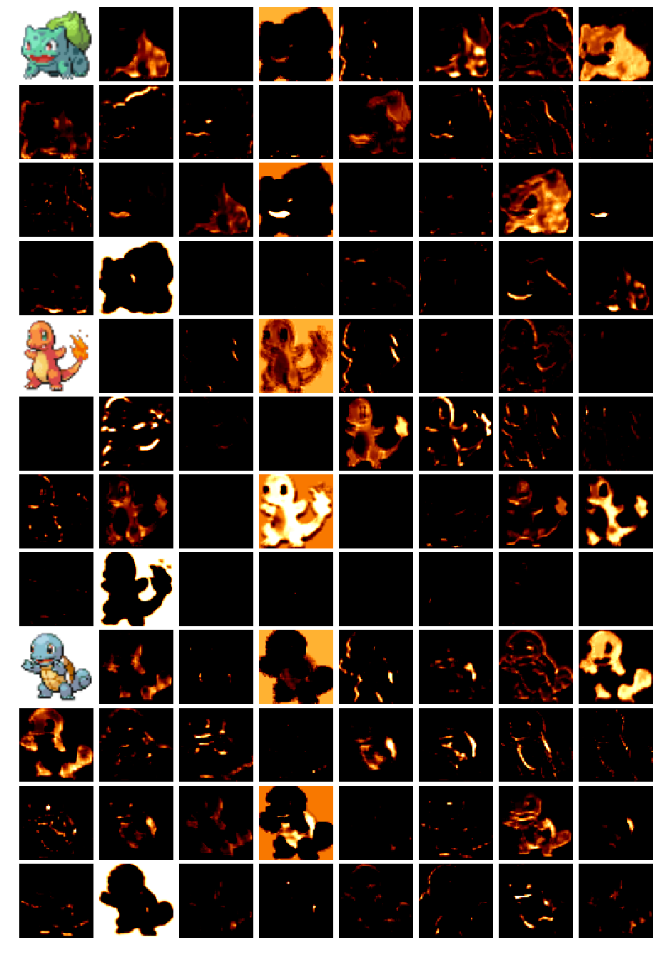
Figure 27. First layer activations (partial) for the three 1^st Gen starters.

CONCLUSION

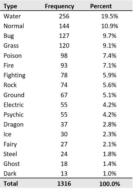
39% accuracy may not seem that impressive. But an 18-class classification problem with as little data as this is a hard one, and our model achieves a 20 percentage points gain against a Zero Rule Baseline, which is to guess the most frequent class for all Pokémon. Table 1 lists the frequencies of each class on the test set, which gives us a 19.5% accuracy for Zero Rule.

Table 1. Type frequency for the test dataset.

But of course, we shouldn’t be measuring our machines against such clumsy methods if we expect them to one day become the dominant rulers of our planet, and computers still have a long way to go if they expect to beat my little brother in the “Pokémon Classification Challenge” someday. On the bright side, they probably already beat my old man. But this is a topic for another article…

REFERENCES

Bulbapedia. (2017) Type. Available from: http:// bulbapedia.bulbagarden.net/wiki/Type (Date of access: 20/01/2017).

Go Game Guru. (2017) DeepMind AlphaGo vs Lee Sedol. Available from: https://gogameguru. com/tag/deepmind-alphago-lee-sedol/ (Date of access: 07/Mar/2017).

Large Scale Visual Recognition Challenge. (2015) Large Scale Visual Recognition Challenge 2015 (ILSVRC2015). Available from: http://image-net.org/challenges/LSVRC/2015/results (Date of access: 20/01/2017).

Scikit-Image. (2017) Module: filters. Available from: http://scikit-image.org/docs/dev/api/skimage.fi lters.html#skimage.filters.sobel (Date of access: 07/Mar/2017).

Tromp, J. & Farnebäck, G. (2016) Combinatorics of Go. Available from: https://tromp.github.io/go/ gostate.pdf (Date of access: 20/01/2017).

Veekun. (2017) Sprite Packs. Available from: https:// veekun.com/dex/downloads (Date of access: 20/01/2017).

Wikipedia. (2017a) Artificial Neural Network. Available from: https://en.wikipedia.org/wiki/ Artificial_neural_network (Date of access: 07/Mar/2017).

Wikipedia. (2017b) Pokémon. Available from: https://en.wikipedia.org/wiki/Pok%C3%A9mon (Date of access: 20/01/2017).

ABOUT THE AUTHOR

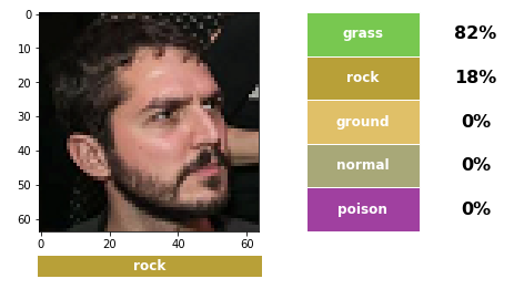
Henrique wants to be the very best, like no one ever was. When he isn’t playing games, devouring sci-fi literature or writing awesome articles to an obscure geek journal on the Internet, he works a full-time job applying machine learning to the banking industry. Sadly, he got misclassified by his own creation. – Grass? Come on!?

Gotta Train ’em All

I wanna be the very best / Like no one ever was

To model them is my real test / To train them is my cause

I will travel across the data / Searching far and wide

Each model to understand / The power that’s inside

Neural Net, gotta train ’em all / It’s you and me / I know it’s my destiny

Neural Net, oh, you’re my best friend / The world we must understand

Neural Net, gotta train ’em all / A target so true / Our data will pull us through

You teach me and I’ll train you

Neural Net, gotta train ’em all / Gotta train ’em all

Yeah

[1] The exact date for the invention of the computer is quite difficult to pin down. Helpful devices for calculations have existed for centuries, but truly programmable computers are a recent invention. If we take as a cutoff criterion that the first computer must be Turing Complete (that is, being able to compute every Turing computable function), our first examples would be placed around the first half of the twentieth century. The first project of a Turing complete machine is attributed to Charles Babbage in the nineteenth century. His Analytical Engine, if ever built, would be a mechanical monstrosity of steel and steam that, although not very practical, would certainly be awesome.

[2] It is estimated that the game space of Go comprises around 2.08·10^170 legal positions or 208,168,199,381,979,984,699,478,633,344,862,770,286,522,453,884,530,548,425,(…)639,456,820,927,419,612,738,015,378,525,648,451,698,519,643,907,259,916,015,628,(…)128,546,089,888,314,427,129,715,319,317,557,736,620,397,247,064,840,935, if you want to be precise (Tromp & Farnebäck, 2016).

[3] Brute force search is a problem-solving strategy that consists in enumerating all possible solutions and checking which solves the problem. For example, one may try to solve the problem of choosing the next move in a tic-tac-toe game by calculating all possible outcomes, then choosing the move that maximizes the chance of winning.

[4] Ideally, we would split our dataset in 3 separate datasets: (1) the ‘training dataset’ would be used to learn the model coefficients; (2) the ‘validation dataset’ would be used to calibrate model hyperparameters, as the learning rate of the training algorithm or even the architecture of the model, selecting the champion model; (3) the ‘test dataset’ would be used to evaluate the performance of the champion model. That way, we avoid introducing bias in our performance estimates due to our model selection process. As we already have a way too small dataset (and we aren’t tweaking the model that much), we can disregard the test dataset.

[5] In machine learning context, an epoch corresponds to an iteration in which all the training data is exposed to the learning algorithm (not necessarily at once). In this case, the neural network learned from 20 successive iterations in which it saw all the data.

[6] I trained all models on Keras using the Tensorflow backend. The training was done in GPU, with a NVIDIA GTX 1080, on a PC running Ubuntu. For more details, see the companion Jupyter Notebook at GitHub (https://github. com/hemagso/Neuralmon).