João Vitor Tomotani
Independent Researcher. São Paulo, SP, Brazil.
Email: tjvitor (at) gmail (dot) com
https://doi.org/10.5281/zenodo.8226232
INVENTORIES IN RPGS AND ADVENTURE GAMES
Video games came a long way to be at where they are today. From the CRT Amusement Devices invented by physicists Thomas Goldsmith Jr. and Estle Mann in 1947, to the OXO / Noughts and Crosses / Tic-Tac-Toe developed by Alexander Douglas in 1952, until we arrive at the Magnavox Odyssey, the first home console created by Ralph Baer in 1972, the same year Atari released its first product, the coin operated Pong (Dillon, 2011).
The story of items and the inventory systems in video games started not long after that. It is probably mandatory, though, to cite the Dungeons & Dragons system of rules, developed by Gary Gigax and Dave Arneson in 1974, as a huge reference. In their system for pen and paper games, Gigax & Arneson (1974) created rules for carrying capacity and encumbrance, which considered the weight of the objects carried (even considering the weight of money in the form of gold pieces, a practice that thankfully is not very popular in games today).
The Dungeons & Dragons system was a huge inspiration for programmer Will Crowther that, in 1976, developed the text adventure game Colossal Cave Adventure. The game was expanded in 1977, with the help of Don Woods, an appreciator of J.R.R. Tolkien and high fantasy elements. In this game, you could type commands to execute actions and interact with objects such as keys and bottles. This interaction included collecting and later using such objects. Colossal Cave Adventure is one of the most influential games of all time, and later had a graphical version developed, Adventure for Atari 2600, famous (among other reasons) for the first “Easter Egg” (Salvador, 2017).
All these adventure and RPG games influenced another wave of games like Akalabeth: World of Doom (1979), Wizardry: Proving Grounds of the Mad Overlord (1981) and Might and Magic Book One: The Secret of the Inner Sanctum (1986), the first games of respectively the Ultima, Wizardry and Might and Magic video game series. Considered the establishers of the computer RPG genre, they further developed the idea of collecting items and using them whenever needed.
From all those popular and influential titles, many other video games and other very famous items and inventory screens appeared. I will talk more about these now and about one of them in particular.
INVENTORY TYPES AND THE VISUAL GRID INVENTORY PROBLEM
There are many different types of video game inventories, and ways these inventories are “limited” by the programmers (DellaFave, 2014).
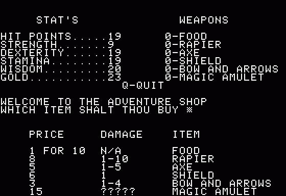
One of the most famous inventory types is the classic “Rule of 99” inventory, usually associated with JRPGs like Final Fantasy, Dragon Quest and Pokémon. This very simple inventory considers that the maximum number of copies you can carry of an item is a specific number defined by the game, usually 99 (though other random numbers may be possible — I am looking at you, Tales series). Also, this inventory type usually considers that all items are shared and can be used freely at any time between all party members (also with some notable exceptions).
Another classic inventory type is the weighted inventory, particularly popular among western RPGs like Fallout and The Elder Scrolls, and in line with the encumbrance rules of Gigax & Arnerson (1974). In the weighted inventory system, each object is assigned a numerical value representing its weight. A character can carry a limited total weight before being affected by a status such as fatigue or reduced movement.
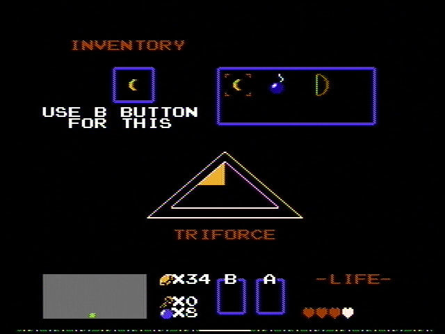
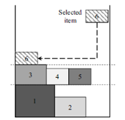
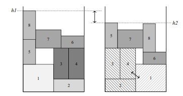
Finally, and most important for this article, there is the visual grid inventory type. In this inventory system, instead of having an infinite amount of space to store items, you have a grid to organize them in. In this inventory system, the size and shape of each item may or may not vary. One example of grid where sizes and shapes do not vary is the Baldur’s Gate inventory system, where curiously a character could carry at most 16 suits of full plate armor or 16 pearls.
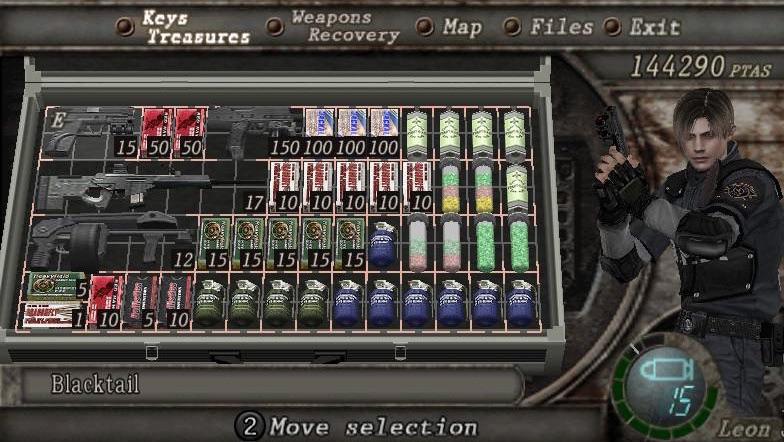
The visual grid inventory system is present in many games, but probably was popularized by the action-RPG Diablo and the survival horror game Resident Evil.
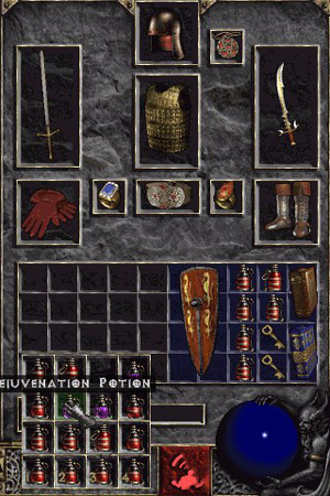
The visual grid inventory brought an interesting dynamic to video games. Now you had limited inventory space and had to plan carefully what was worth bringing to underground dungeons or to the zombie apocalypse — a small dose of realism in worlds full of demons or zombies.
Organizing your equipment became a challenge on itself, and a challenge well studied by academics, as we will see.
THE TWO-DIMENSIONAL KNAPSACK PROBLEM
The Knapsack Problem is a classical problem in combinatorial optimization, being part of the broader class of Cutting and Packing (C&P) problems. In the Knapsack Problem, a set of entities are given, each having a value and a size, and the objective is to select one or more entities so that the sum of the sizes does not exceed a given limit (the size of the knapsack), while the sum of the values of the selected entities is maximized (Martello & Toth, 1990). Knapsack problems have been studied by academics and practitioners for over a century, being able to model many industrial (and survival horror) situations. For instance, Salkin & de Kluyver (1975) discussed its many different applications in industrial situations such as cargo loading, project selection, and budget control, while also presenting others, like capital budgeting and selecting journals in a library. But no mention was made on how to select equipment for a survival horror scenario.
A mathematical formulation of the knapsack problem is:

where xj is the binary variable that defines whether item j is “placed in the knapsack” or not; pj is the profit obtained by placing item j in the knapsack; rij is the units of resource i consumed by placing item j in the knapsack; and bi is the limit available (or budget) of resource i. As can be seen by this formulation, it is possible to have different constraints (also called knapsack constraints), so that this problem can be called multidimensional knapsack problem (MKP), m-dimensional knapsack problem, multiconstraint knapsack problem, among other names (Chu & Beasley, 1998).
The “simple” knapsack problem is very similar to the weighted inventory dilemma a player faces when deciding which items to carry. Each item has a different numerical value attributed to it, representing its weight or size, and we, the players, internally and empirically evaluate each item’s usefulness, and attribute to them a value (or profit).
This “simple” knapsack problem is also known as one-dimensional knapsack problem. A variation of this problem considers that, instead of a subset of items with one or more one-dimensional constraints represented by a single number, the items instead are a subset of shapes that are to be packed into a larger shape (or multi-dimensional knapsack if you will). The most studied version of this problem is the orthogonal two-dimensional knapsack problem (2KP), where the input consists of a set of n small rectangles (thus “orthogonal”), each with their own width w, height h and profit p, to be placed without overlaps into a large rectangle of width W and height H, aiming to maximize the total sum of profits P. While the one-dimensional knapsack problem is known to be solvable in pseudopolynomial time by dynamic programming, the 2KP is strongly NP-hard (Caprara & Monaci, 2004).
Box 1. NP-Hardness.
In computational complexity theory (field in theoretical computer science and mathematics, that studies and classifies problems according to their resource usage when trying to solve them computationally), NP (non-deterministic polynomial time) is a complexity class used to classify decision problems – problems with a yes/no answer.
A decision problem is classified as P (polynomial time) if it can be solved “quickly” (note that we use the term “quickly” VERY lightly here), that is, if there is an algorithm that can solve this problem in polynomial time (as opposed to, for example, exponential time).
On the other hand, a decision problem is classified in NP if, given a candidate answer to the problem, it can be verified in polynomial time (there are also other complicated definitions here for NP problems, that involve solving them in polynomial time using nondeterministic Turing Machines, but we will not go down this path).
A practical example of a NP problem is a Sudoku. The decision problem (yes/no problem) can be: “given a sudoku puzzle, does it have a solution?” It may take a long time to find this answer. On the other hand, if the solution for the Sudoku is given, verifying whether the solution is correct is much quicker.
Other classic example is the problem of integer factorization – that is, the decomposition of a composite number into a product of smaller integers. Factoring the number is a very hard problem. But verifying whether a solution is true is as simple as multiplying the factors and confirming the solution.
A problem is classified as NP-hard, if it is at least as hard as the hardest problem in NP.
By considering the geometry and the orientation of the pieces (or, in our definition, items), additional complexities can be added to the problem. Bortfield & Winter (2009) made a list of possible constraints and classified previous studies considering two criteria: (1) the type of stock of pieces: unconstrained knapsack problem, where the number of copies per type is not fixed; constrained knapsack problem, where there is an upper limit of copies allowed; and doubly constrained knapsack problem, where both an upper and lower limit of copies per piece are defined; and (2) the problem subtype: orientation constraint, whether pieces can be rotated or not; and a guillotine cutting constraint, that considers whether pieces can be reproduced through a guillotine cut – this is more specific to the Cutting and Packing class of problems (C&P; see Box 2), to which the knapsack problem is a subtype.
Most studies on the two-dimensional knapsack problem consider only rectangular shapes (orthogonal two-dimensional knapsack problem, or 2KP). There is also a variation of this problem that consider the existence of irregular shapes, like the study from Del Valle et al. (2012). The present article will not consider this much more complicated variation, though I advise that in case of a zombie apocalypse, all optimization is valid.
Box 2: Cutting and Packing Problems.
Cutting and Packing problems (C&P) is the name given for a broad range of problems that follow a similar logical structure, under different names, in the literature. Some examples are cutting stock and trim loss problems; bin packing, strip packing, vector packing, knapsack problems; vehicle loading, pallet loading, container loading problems; and capital budgeting and memory allocation problems. With few exceptions, scientific work on this topic started around the 1960s, with a fast-growing volume of articles dealing with different variations of the C&P in management science, engineering science, information and computer sciences, mathematics and operational research fields (Dyckhoff, 1990).
Dyckhoff (1990) classified the C&P according to several other characteristics: Dimensionality (whether one or more dimensions of the geometry are considered); Quantity measurement (if the dimensions are discrete or continuous); Shape of figures (form, size, orientation, regular or irregular forms); Assortment (shape and number of the permitted pieces); Availability (lower and upper bounds of quantities for each piece, sequence orders for the placement of pieces, dates to be cut or packed); Pattern restrictions (minimal distance between pieces, frequency and orientation of small pieces); Assignment restrictions (number of assignment stages, number, frequency or sequence of patterns, dynamics of allocation); Objectives of the C&P; Status of information and variability (problem data is deterministic, stochastic or uncertain, and whether the data is strict or may be variable).
ZOMBIE APOCALYPSE INVENTORY MANAGEMENT HEURISTICS
In this article, I explore solutions to the two-dimensional knapsack problem as applied to Resident Evil, hoping to aid people during virtual zombie apocalypses. But before we start, we need a crash course in heuristics.
Heuristics are techniques designed for problem solving, based on previous experiences and knowledge from similar problems. Heuristics employ a practical method, aiming to provide a good enough solution for the problem at hand within a reasonable time. They are not guaranteed to find an optimal solution, though, and are not able to recognize an optimal solution if one is found; also, no distance to the optimal solution can be computed or guaranteed.
Heuristic algorithms are usually divided into constructive heuristics and improvement heuristics. Constructive heuristics build solutions by adding elements until the solution is completed, or the process is interrupted or finished with no feasible solution found. Improvement heuristics, on the other hand, start with an initial solution – a complete solution obtained by a constructive heuristic or a randomly generated one – and this initial solution is improved by applying small consecutive changes, until a stopping criterion is met. Oliveira et al. (2016) discussed the existing heuristics applied to the two-dimensional rectangular strip packing problem (a problem within the C&P problems), classifying them as follows (this is a very brief summary of some of the methods, a much more extensive literature review is made by Oliveira et al., 2016[1]).
Constructive heuristics
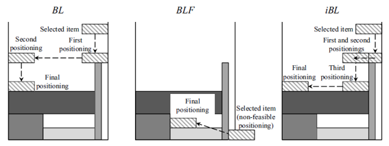
- Positioning-based heuristics: the oldest heuristics in academic literature. They are flexible and able to incorporate most usual constraints of the problem. The Bottom-Left heuristic (BL), proposed by Baker et al. (1980), was the first positioning-based heuristic ever proposed and the most well-known (Oliveira et al., 2016). This heuristic is very fast, but as a drawback is unable to fill “holes”, or empty spaces surrounded by pieces. Many heuristics were proposed to solve this issue; one of the most famous is the Bottom-Left-Fill (BLF) proposed by Chazelle (1983). The BLF consider all empty spaces as admissible for placing new pieces, even when surrounded by other pieces, and always results in solutions that are equal to or better than the BL. This search for empty feasible spaces, though, is much more complex and demanding of computational time. Finally, the Improved Bottom-Left (iBL) proposed by Liu & Teng (1999) always prioritize the down movement over the left movement, moving only the necessary minimum to the left when moving down is not possible.
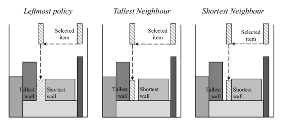
- Fitness-based heuristics: these heuristics focus on the empty spaces, searching for the best-fit between the piece to be placed and the empty spaces available. The Best-Fit heuristic (BF) proposed by Burke et al. (2004), for example, locates the lowest free space available, then searches for a piece that will perfectly fit that space. If there is no such piece, then the next largest piece that fits the space is chosen and placed. The location of the placement can also have different rules: leftmost policy, next-to-tallest policy, or next-to-shortest-policy.
- Level-based heuristics: these heuristics are very different from the previous two types, addressing a specific real-world problem where the level orientation of the layouts is a constraint, for instance when planning display of goods on supermarket shelves (Oliveira et al., 2016). The strategy for these heuristics is to place the pieces on parallel levels, where the height of each level is defined by the tallest rectangle placed on it. One example is the heuristic proposed by Coffman Jr et al. (1980), the Next-Fit Decreasing Height (NFDH), in which rectangles are sorted by non-increasing height, and placed one at a time on the current open level, in the leftmost position, until there Is not enough space to accommodate a new rectangle, and a new layer is opened. As mentioned, level-based heuristics address specific real-world problems, but has the limitation of not necessarily being ideal to optimize space in a knapsack for an end-of-world crisis.
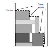
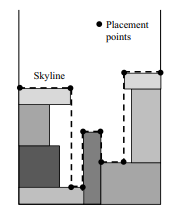
- Profile-based heuristics: the profile or contour is a concept introduced by Scheithauer (1997), consisting of a polygonal line starting from the left side of the large rectangle where the pieces are being placed, and ending on the bottom or right side of it, composed by vertical and horizontal edges. This concept was first introduced to build exact methods, but later its potential for developing heuristics was identified by other authors. One example is the study of Wei et al. (2011) that proposed the “Iterative Doubling Binary Search” heuristic (IDBS). In that work, a profile (called skyline) composed of the edges or extension of edges of already placed rectangles defined the feasible placement points. Then, the IDBS analyzed where to place the next rectangle, according to several criteria using a scoring method.
Improvement heuristics
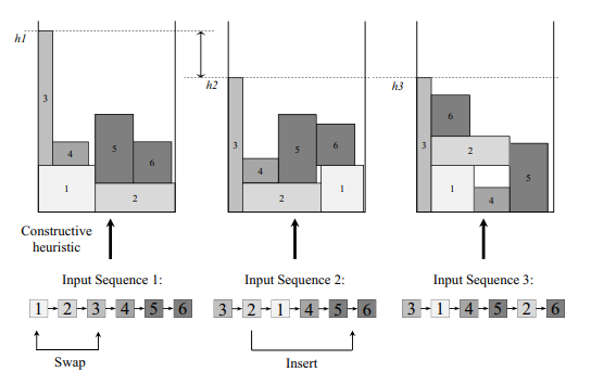
- Search over sequences: improvement heuristics based on the search over sequences strategy resort to modifications to the used sequence as the basis for the constructive heuristic. There are two different operations, the insert operation – where a rectangle is taken out of the sequence and re-inserted in a different position – and the swap operation – in which two rectangles exchange their positions in the sequence. The most basic search strategy is the Local Search (LS), in which an incumbent solution is tested and, if better than the current “best solution”, accepted. The search stops when a previously defined number of changes are tested without improvement to the solution. Pure local search methods are known for getting stuck in local minima (solutions that are better than any other solution that can be generated from it, but with no guarantee of global optimality) and, because of that, it is common for them to be combined with metaheuristic methods, like genetic algorithms, tabu search, or simulated annealing, to avoid being stuck in those solutions.
- Search over layout: in this improvement heuristic, modifications are operated directly over the layout of the solution, changing the position of two or more pieces based on their current placement. One example is the algorithm proposed by Alvarez-Valdes et al. (2005), which defines a fitness value for each piece, based on how well it occupied the space, and then uses this value to define candidates to be replaced.
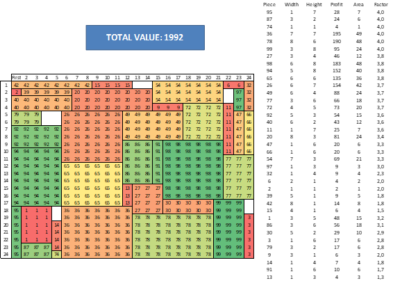
TESTING HEURISTICS FOR THE RESIDENT EVIL INVENTORY MANAGEMENT PROBLEM (REIMP)
One important difference of the proposed Resident Evil Inventory Management Problem (REIMP) when compared to typical C&P explained above, is that C&P usually focuses on minimizing the space occupied in a deposit when placing all pieces (henceforth called “items”), instead of maximizing the profit by placing only a limited amount of items. The two-dimensional rectangular strip packing problem considers that the “container” has all dimensions but one fixed (in other words, the “height” of the deposit is limitless), and the idea is to minimize the height of the configuration of pieces, while pieces can be stacked indefinitely. As such, there is no need to consider the concept of “profit” of each item since all of them must be placed. In the REIMP, however, the value empirically attributed to each item is important and must be considered for the best solution.
The characteristics of the REIMP are:
- The items are all rectangular, with sides varying from 1 to 8 units of length, with only integer values allowed. The items cannot change their orientation (cannot be rotated). Though the non-rotation premise differs from what is possible in RE, this was considered to simplify the problem;
- Each item is assigned a “profit” value. The profit of each item is proportional to its area, to avoid having very small items with very large values, which could skew the quality of the analysis. The profit is an integer value, and is calculated by multiplying the area of the item by a random factor between 1 and 4 (not necessary an integer factor);
- The 2D knapsack (henceforth called “inventory” as per common sense) is a square of side of 24 units of length. The size of the knapsack is variable, and this square of 24 units of length is obviously different from the inventory in RE, but the knapsack problem can be changed in our program;
- 100 items each were generated randomly, and the objective of the REIMP is to maximize the total profit of items placed in the inventory;
- Other 2KP characteristics apply, such as: items cannot overlap; items cannot be placed partially; items can be placed next to each other with no gaps.
For this problem, the following heuristics were tested:
- Bottom-Left Heuristic (BL);
- Improved Bottom-Left Heuristic (iBL);
- Improvement Heuristic based in the search over sequence technique, that consists of reordering the priority that the pieces of a first solution are tested, based on the height of the pieces (IH). This improvement heuristic was applied to the solutions obtained by the BL (IHBL) and iBL (IHiBL). Strictly speaking, this is technically not really an improvement heuristic, since it does not consist of small and consecutive changes being applied to an existing solution until a stopping criterion; rather, it is more in line with a new priority rule for a new constructive heuristic;
- A routine that filled gaps once a first solution was defined, using a “brute force” approach (FG). This routine was possible due to the small size of the problem. This improvement was applied to the solutions obtained by the BL (FGBL) and iBL (FGiBL).
For the testing, 10 instances of 100 items each were generated. For each instance, the six heuristics were tested: BL, iBL, IHBL, IHiBL, FGBL, and FGiBL. The problem was modeled in VBA.
Since it is not possible to fit all items in the inventory, it is necessary to define the order that the pieces are tested and placed, or their priority. For this, all heuristics considered that the “Factor” of each item can be considered as the priority for that item (the factor being the profit divided by the area). In case of two items having the same factor, the tiebreaker was the area – the larger ones being tested first.
A disadvantage of this strategy is that testing the items according to their factor guarantees that we are prioritizing items according to their profit to area ratio, but we are not looking into their shape. As such, there will be situations where large empty spaces are formed, since items with very different sizes are placed side to side. This can be mitigated by our Improvement Heuristic (IH), which changes the orders that the shapes are placed. Once a solution was found for the BL and iBL, this IH was applied to both (IHBL and IHiBL, respectively). This heuristic considered all the items that made the first solution, and reorganized them according to their height. Once this new order is defined, the same constructive heuristics are performed, considering this new order. This solution improved the organization of the pieces, reducing empty spaces. Then, once all previously placed items are placed again, the items that did not manage to fit the first solution are tested again, according to their factor.
Finally, the FG heuristic was applied to both the BL and iBL solutions. As mentioned before, this brute force approach checks all remaining pieces in order of their factor, and all empty spaces, trying to fit the remaining pieces.
The figures below show these six heuristics tested for one of the instances of the problem. Finally, the Table 1 shows the results obtained for the ten instances.
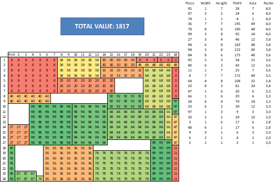
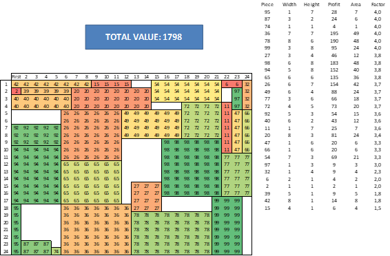


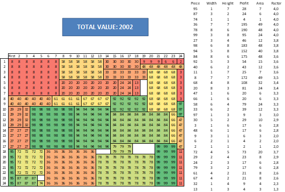
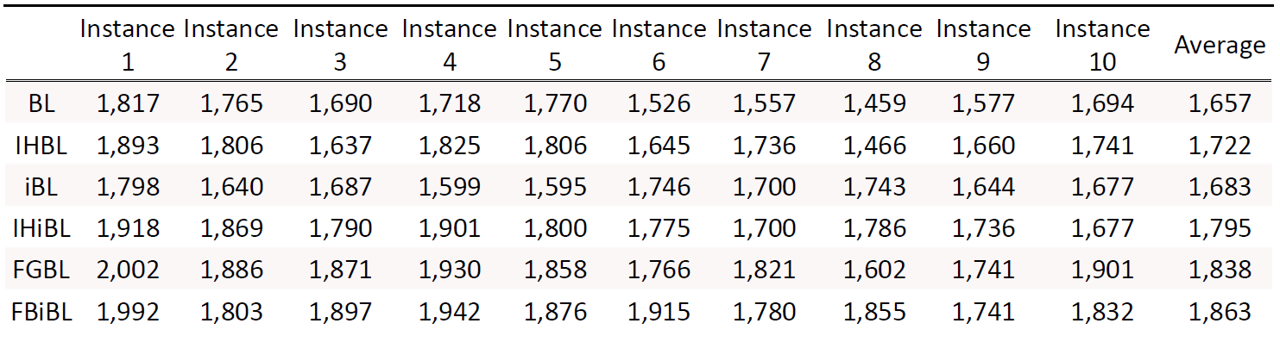
As can be seen in Table 1, for all cases but one, the Improvement Heuristic provided better or equal results than the original solution they started with. Comparing the BL and iBL heuristics, though, it is unclear which performs better with only ten instances of relatively small size; it depends on the configuration of the items. Finally, the FG routine presented better results with very few exceptions. Since this routine only tries to place additional items in the empty spaces, it will never present a worst result than the original ones and could be used after the IHBL or IHiBL.
Additional ideas could be tested to improve upon these results. For instance, heuristics that delete one of the items from the inventory – possibly the largest one – to see if the new arrangement reduces the number of empty spaces.
CONCLUSION
As I discussed in a previous study (Tomotani, 2015), a zombie outbreak would probably have very damaging effects to human society as we know. Considering this, it is very important to know different optimization techniques that can be useful when planning for apocalyptic scenarios. Curiously, very few optimization studies focus on said scenarios, instead prioritizing industrial and supply chain problems to maximize profit. I emphasize that dealing with a zombie apocalypse capable of ending humanity is probably an issue as relevant as making rich people even richer and propose that more efforts should be directed to this area.
REFERENCES
Alvarez-Valdes, R.; Parreño, F.; Tamarit, J.M. (2005) A GRASP algorithm for constrained two-dimensional non-guillotine cutting problems. Journal of the Operational Research Society 56(4): 414–425.
Baker, B.S.; Coffman Jr, E.G.; Rivest, R.L. (1980) Orthogonal packings in two dimensions. SIAM Journal of Computing 9(4): 846–855.
Bortfeldt, A. & Winter, T. (2009) A genetic algorithm for the Two-dimensional Knapsack Problem with rectangular pieces. International Transactions in Operational Research 16: 685–713.
Burke, E.K.; Kendall, G.; Whitwell, G. (2004) A new placement heuristic for the orthogonal stock-cutting problem. Operations Research 52(4): 655–671.
Caprara, A. & Monaci, M. (2004) On the Two-dimensional Knapsack Problem. Operations Research Letters 32: 5–14.
Chazelle, B. (1983) The Bottomn-Left Bin-Packing Heuristic: An Efficient Implementation. IEEE Transactions on Computers C-32(8): 697–707.
Chu, P.C. & Beasley, J.E. (1998) A genetic algorithm for the Multidimensional Knapsack Problem. Journal of Heuristics 4: 63–86.
Coffman Jr, E.G.; Garey, M.R.; Johnson, D.S.; Tarjan, R.E. (1980) Performance bounds for level-oriented two-dimensional packing algorithms. SIAM Journal on Computing 9(4): 808–826.
Del Valle, A.M.; Queiroz, T.A.; Miyazawa, F.K.; Xavier, E.C. (2012) Heuristics for two-dimensional knapsack and cutting stock problems with items of irregular shape. Expert Systems with Applications 39(16): 12589–12598.
DellaFave, R. (2014) Designing an RPG Inventory System That Fits: Preliminary Steps. Available from: https://gamedevelopment.tutsplus.com/articles/designing-an-rpg-inventory-system-that-fits-preliminary-steps–gamedev-14725 (Date of access: 06/Feb/2022).
Dillon, R. (2011) The Golden Age of Video Games. Routledge, London.
Dyckhoff, H. (1990) A typology of cutting and packing problems. European Journal of Operational Research 44(2): 145–159.
Gigax, G. & Arneson, D. (1974) Dungeons & Dragons. Tactical Study Rules, Lake Geneva.
Hopper, E. & Turton, B.C.H. (2001) A review of the application of meta-heuristic algorithms to 2D strip packing problems. Artificial Intelligence Review 16: 257–300.
Liu, D. & Teng, H. (1999) An improved BL-algorithm for genetic algorithm of the orthogonal packing of rectangles. European Journal of Operational Research 112(2): 413–420.
Martello, S. & Toth, P. (1990) Knapsack Problems: Algorithms and computer implementations. John Wiley & Sons, West Sussex.
Oliveira, J.F.; Neuenfeldt Júnior, A.; Silva, E.; Carravilla, M.A. (2016) A survey on heuristics for the two-dimensional rectangular strip packing problem. Pesquisa Operacional 36(2): 197–226.
Salkin, H.M. & de Kluyver, C.A. (1975) The Knapsack Problem: a survey. Naval Research Logistics Quarterly 22(1): 127–144.
Salvador, R.B. (2017) History’s first Easter egg. Journal of Geek Studies 4(2): 63–68.
Scheithauer, G. (1997) Equivalence and dominance for problems of optimal packing of rectangles. Ricerca Operativa 83: 3–34.
Tomotani, J.V. (2015) Modeling and analysis of a Zombie Apocalypse: zombie infestation and combat strategies. Journal of Geek Studies 2(1): 10–25.
Toth, P. (1980) Dynamic programming algorithms for the Zero-One Knapsack Problem. Computing 25: 29–45.
Wei, L.; Oon, W.C.; Zhu, W.; Lim, A. (2011) A skyline heuristic for the 2D rectangular packing and strip packing problems. European Journal of Operational Research 215(2): 337–346.
About the author
João Tomotani, MSc., is an engineer that works with Supply and Inventory Planning (or, as he likes to put it, Excel spreadsheets). He is terrible with horror and survival horror games, movies, books, etc., and would definitely be one of the first to die in case of a zombie outbreak.
[1] Those authors also briefly comment on metaheuristics applied to the C&P problems, but a more specific review on metaheuristics is made by Hopper & Turton (2001), where tabu search, simulated annealing, genetic algorithms, among other metaheuristics applied to the 2D Strip Packing Problems, are discussed.

